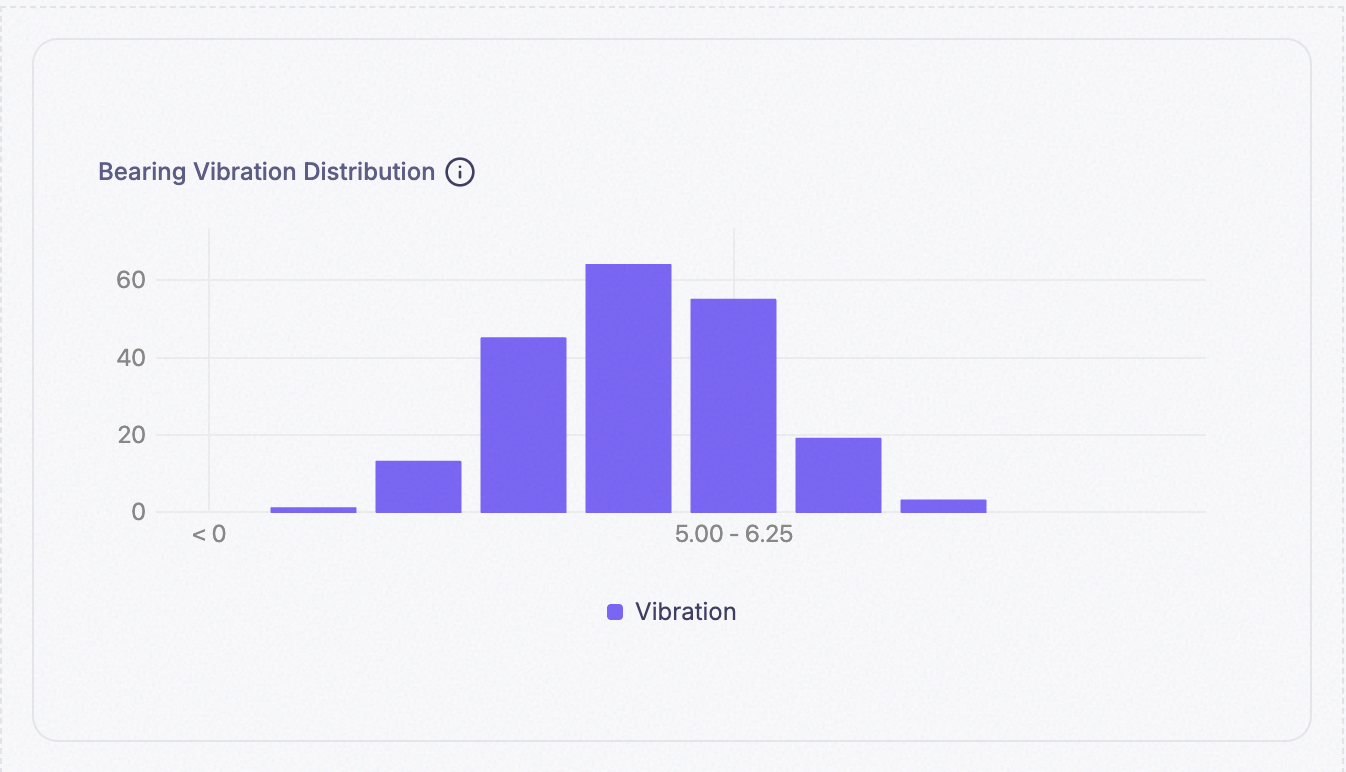
6. Histogram Widget
Shows how often a reading fell into each of several value ranges. Where a Graph plots a value against when it happened, Histogram deliberately throws the “when” away and plots it against how often — the widget for “was this sensor mostly running warm, or mostly cool with the occasional spike,” a question a line chart can technically answer but a distribution answers at a glance. It’s a two-step widget: first it slices your Time Range into buckets the same way a Graph does, using Interval — then it counts how many of those bucketed values landed in each value range you define below.
- Examples:
- A histogram showing the distribution of hourly-average temperatures over the last week.
- A histogram displaying how often different humidity levels occurred.
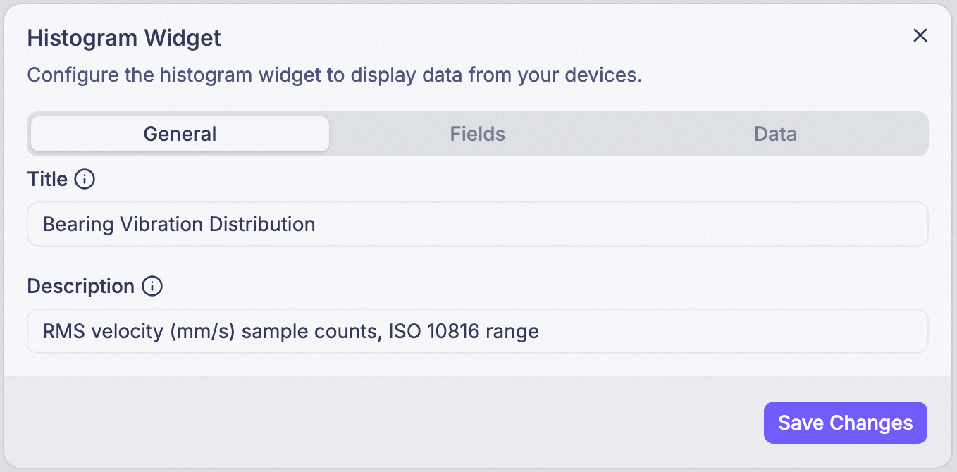
Step 1: Set Title and Description
Title is what’s actually displayed as the widget’s heading. Description isn’t shown on the card at all — it only appears in a tooltip when someone hovers the info icon (ⓘ) next to the title.
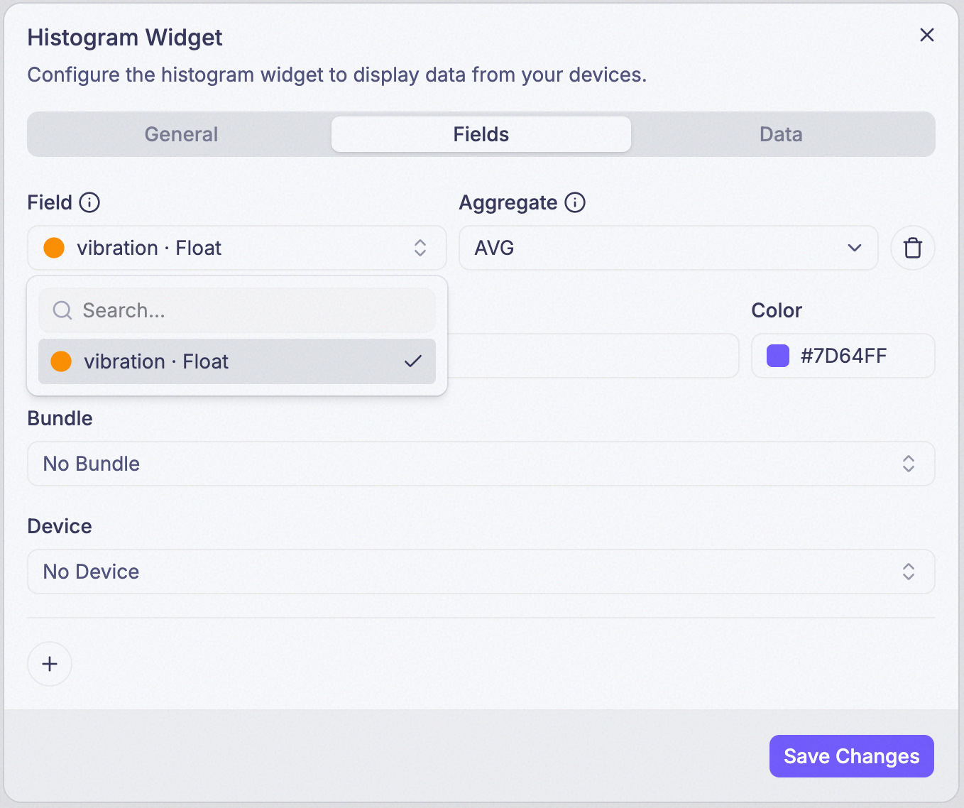
Step 2: Add a Field
Only numeric fields can be picked here. A Histogram can plot more than one field, each with its own settings below.
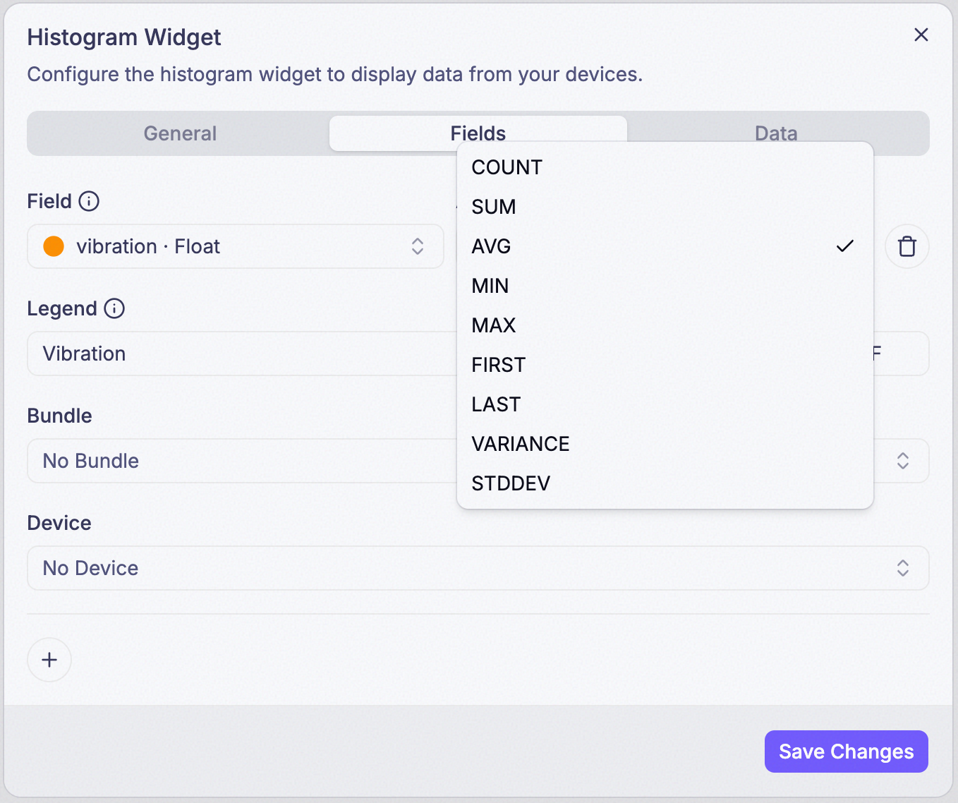
Step 3: Choose an Aggregate for the field
Aggregate decides which single number represents this field inside each time bucket:
| Mode | Shows |
|---|---|
COUNT | How many readings arrived |
SUM | All readings added together |
AVG | The average of all readings |
MIN | The lowest reading |
MAX | The highest reading |
FIRST | The earliest reading inside the bucket |
LAST | The most recent reading inside the bucket |
VARIANCE | Statistical variance of the readings |
STDDEV | Standard deviation of the readings |
No LATEST here — a bucket needs a value regardless of when it was read, not just the most recent one,
so LATEST isn’t offered.
Step 4: Set Legend and Color
Legend is how this field is named if you ever add a second one. Color is its color in the chart.
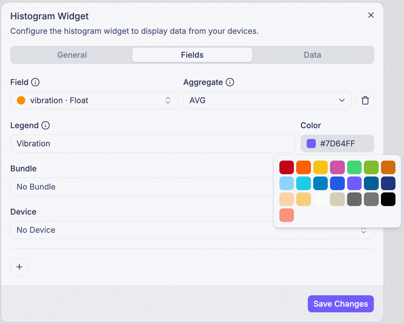
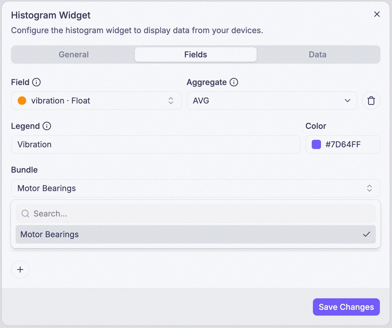
Step 5: Choose a Bundle (optional)
Points this field at every device in a bundle instead of one device. Leave it blank to pick a single device instead, in the next step.
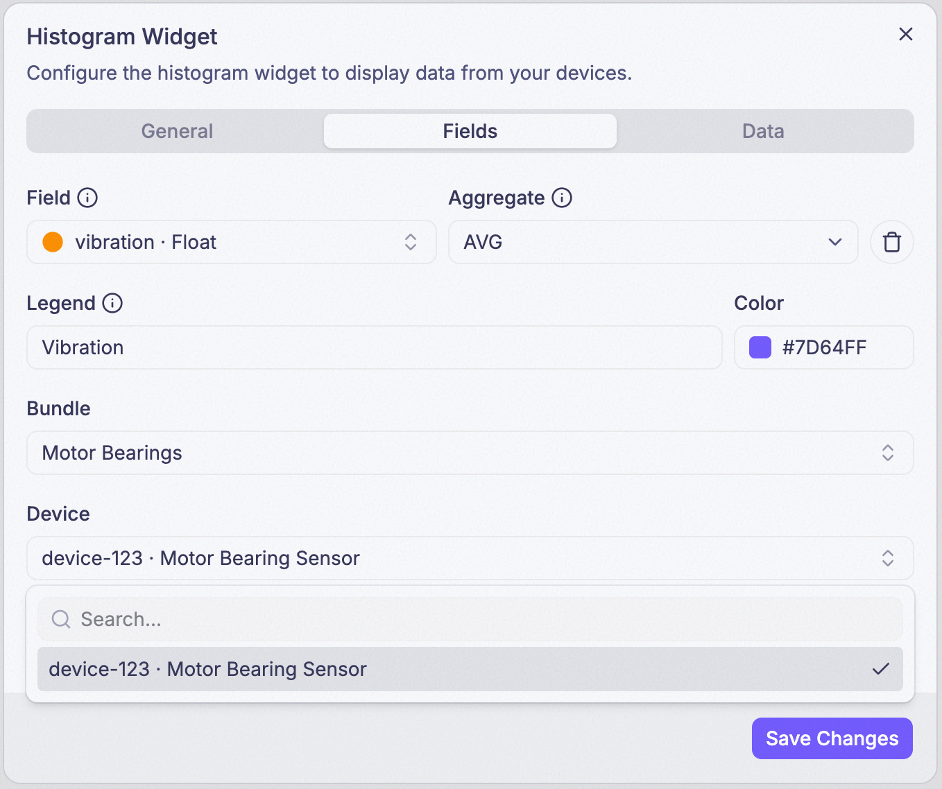
Step 6: Choose a Device (optional)
Points this field at one specific device. Leave both Bundle and Device blank and it reads from any device that reports the field.
Step 7: Move to the Data tab
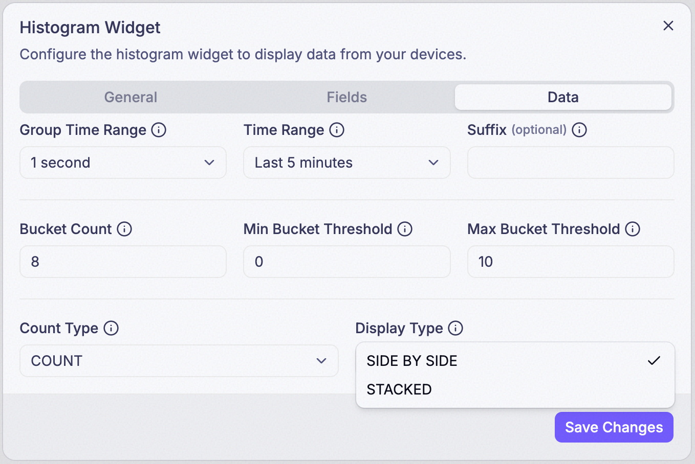
Everything from here on applies to the widget as a whole, not to one field.
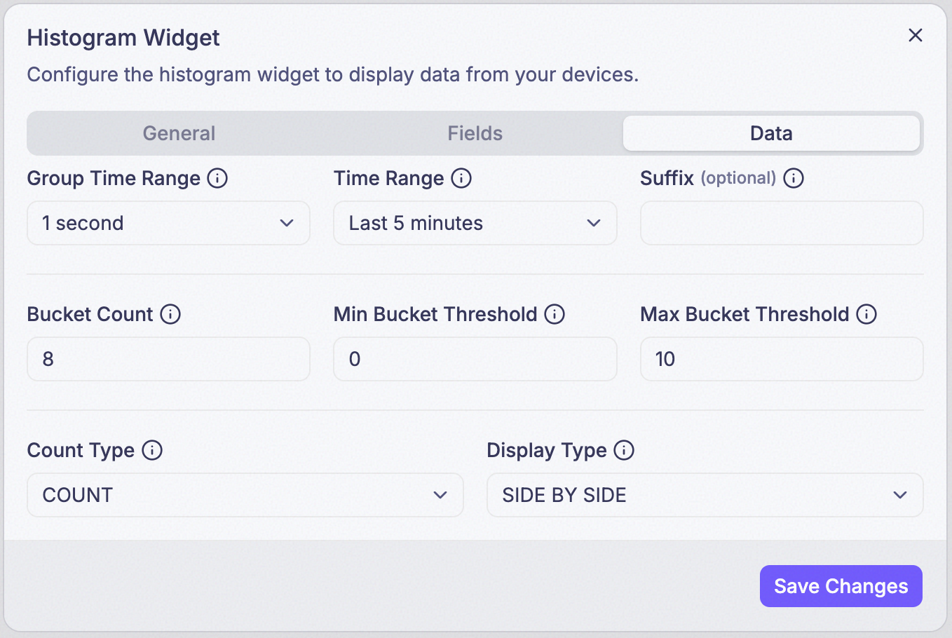
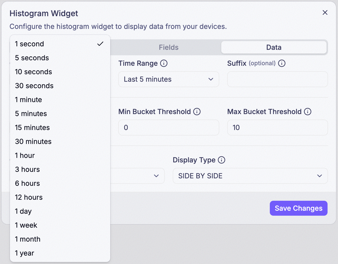
Step 8: Set Interval
Slices the underlying data into time buckets, exactly as on a Graph — a 1-hour Interval averages (or sums, or counts, depending on Step 3) every reading within each hour into a single bucketed value before Histogram ever looks at value ranges.
Step 9: Set Time Range and Suffix
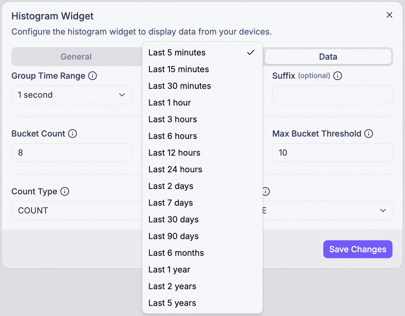
Time Range is the overall period the underlying time series covers. Suffix (optional) is a unit appended to the values shown on the chart (e.g., “°C”).
Step 10: Set Bucket Count, Min Bucket Threshold, and Max Bucket Threshold
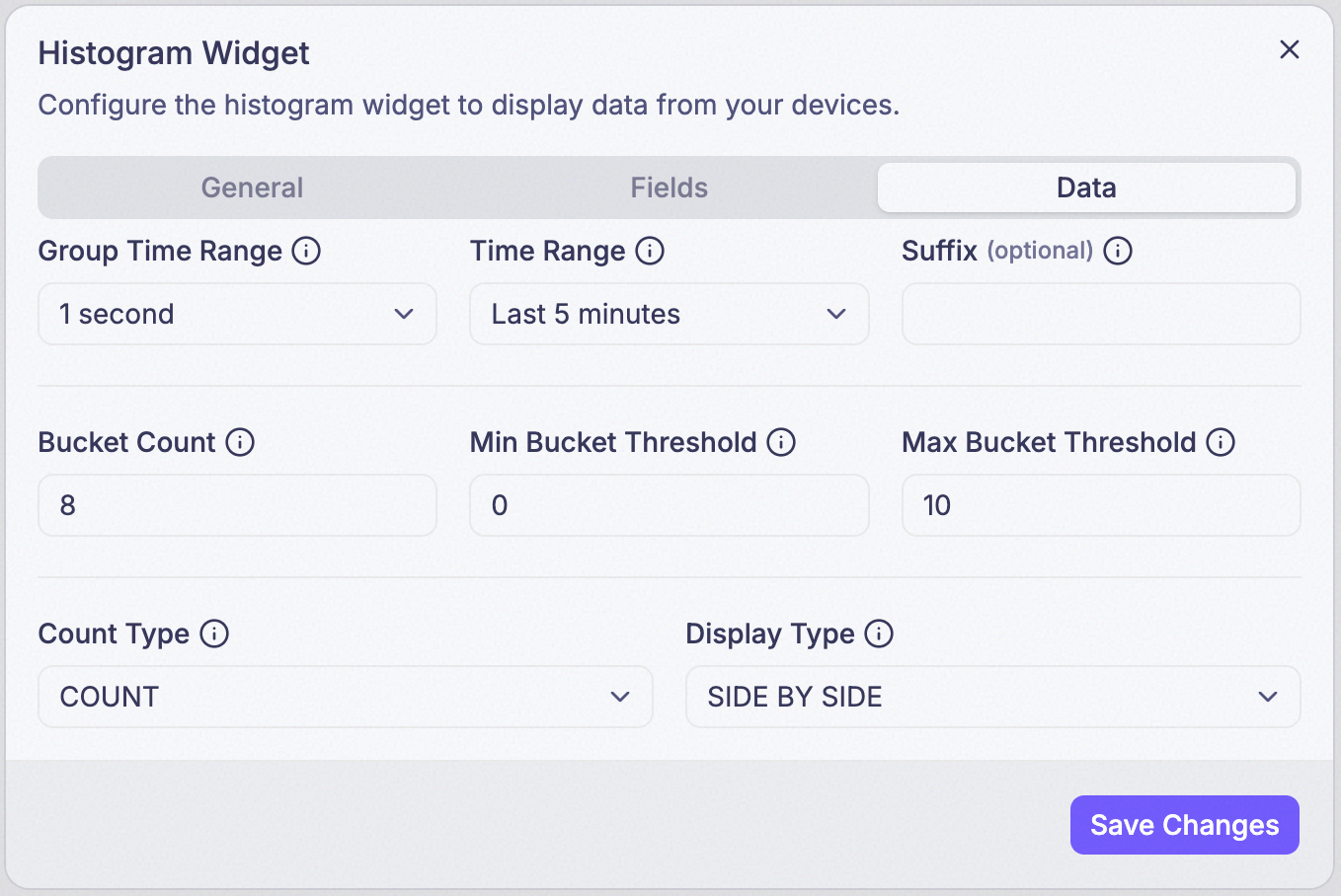
Bucket Count is how many value ranges to split into — the editor allows 1 to 10. Anything below Min Bucket Threshold is folded into the first bucket; anything above Max Bucket Threshold is folded into the last one. Max must be greater than Min.
Step 11: Set Count Type
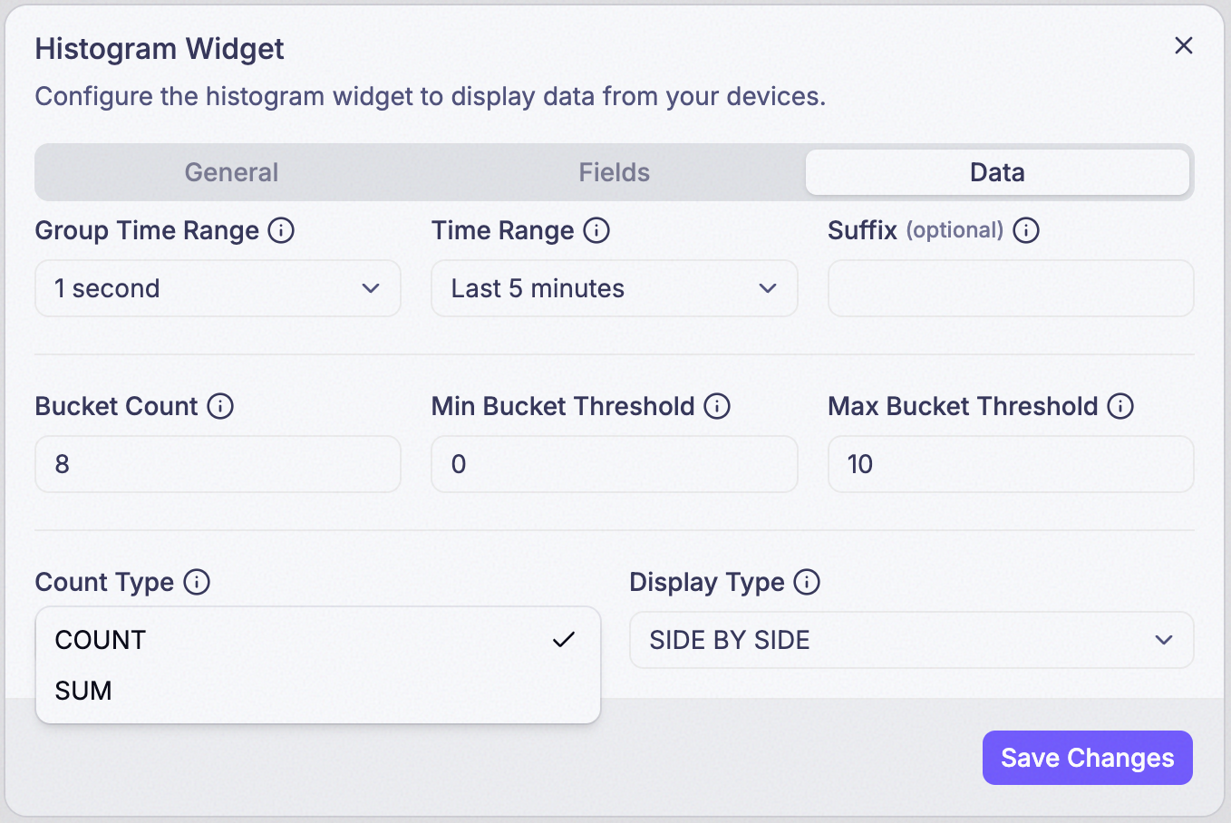
COUNT shows how many bucketed values landed in each range. SUM shows their total instead.
Step 12: Set Display Type
SIDE BY SIDE or STACKED — only matters once the widget has more than one field.
Because Histogram builds its time series the same way Graph does, the same roughly-3,000-point ceiling from the Graph Widget applies here too — a very fine Interval over a very long Time Range can refuse to save for the same reason.
Example